2 Minimum Viable Mathematics

In the corporate world, the term “minimum viable product” (MVP) refers to a product with just enough features to satisfy early customers and provide a base that you can build upon. In the same spirit, here we present the “minimum viable mathematics” that will allow you to build an intuitive understanding of how transformers can “think” by representing ideas as vectors and composing and operating on them.

2.1 Vectors

Vectors are just mathematical objects that form a nice “space” such that any member of the space can be scaled up or down by any constant factor, and any two members of the space can be added together. The result of these operations, or any combination of many such operations, is always another member of the same space. The key point is that the result is always the same type of object that you started with, you never get some different type of object that you don’t know how to handle or interpret. This allows you to compose vectors in arbitrarily complex and subtle ways. Or, conversely, to take some complicated vector and decompose it into a sum of contributions from simpler vectors that we understand better. These are incredibly useful, and fundamental, properties for a mathematical model of any system. Unsurprisingly, vector spaces show up in countless applications in math and science.

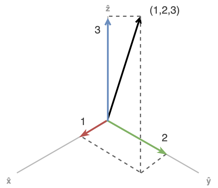
The prototypical example in \(\mathbb{R}^n\), the space of n-dimensional vectors of real numbers. Vectors are imagined as either points in the space, or as arrows from the origin to that point. For example, consider the vector \((1,2,3)\) in three-dimensional space. We can decompose this into a sum of three terms: \(1 \cdot \hat{x} + 2 \cdot \hat{y} + 3 \cdot \hat{z}\), where \(\hat{x}\), \(\hat{y}\), and \(\hat{z}\) are the unit vectors along the x, y, and z axes, respectively. We can decompose any vector in the space into 3 simple terms, one for each of the x-, y-, and z-axes. So if we “understand” each of the three “axes” in three-dimensional space, we can compose them into any vectory in that space; if we are given an arbitrary vector in the space, we can decompoose it into the simpler units along the axes.

Figure 2.1: Decomposing the vector (1,2,3) into its basis components along the x, y, and z axes.

However, many other types of objects besides lists of real number can be shown to form a vector space, including certain classes of polynomials, equations, functions and matrices. Additionally, when we use vectors to represent abstract concepts or real world objects, then we can reason about and compute on these concepts with vector operations. As a concrete example, in early physics classes you learn to draw and interpret “free body diagrams”, where every force acting on some object is represented as a vector. These diagrams can be used to describe a weight on an inclined plane or the lift, gravity, thrust and drag forces on an aircraft, for instance. The total force is the vector sum of all the forces, and allows you to determine whether the block will slide up or down and the aircraft will fly or crash. Conceptually, we think of “adding forces”, but mechanically we are doing vector addition.

Formally, there are eight axioms that a vector space must satisfy. If you can define some class of objects and operations on them that obey these rules, then all the properties and theorems about vector spaces will be true for your class of objects and operations. You don’t really need to know them, but for completeness, here they are:

There are four rules for vector addition:

Commutativity: \(u + v = v + u\)
Associativity: \(u + (v + w) = (u + v) + w\)
Identity element: There exists a zero vector \(0\) such that \(v + 0 = v\) for all \(v\)
Inverse element: For every vector \(v\), there exists a vector \(-v\) such that \(v + (-v) = 0\)

and four rules for scalar multiplication:

Compatibility: \(a(bv) = (ab)v\) This is just associativity of scalar multiplication
Multiplicative identity element: There exists a scalar \(1\) such that \(1v = v\) for all \(v\)
Distributivity over vector addition: \(a(u + v) = au + av\)
Distributivity over scalar addition: \((a + b)v = av + bv\)

Essentially, these just ensure that the addition and multiplication obey all of your intuitions about how they changing parenthesis, order, etc. affect addition and multiplication of integers or real numbers. In this book we will only work with \(\mathbb{R}^n\) vector spaces.

Important

Vectors are objects that compose nicely within a “space” of all such objects.
Since rescaling a vector or adding vectors always results in a valid vector, you can mix as many vectors as you like, in whatever proportions you like, to create new vectors.
Conversely, you can always take any vector and decompose it into a weighted sum of simpler vectors that you understand or know how to work with.
This ability to mix vectors representing different concepts is crucial for modeling nuanced concepts.

2.2 Dot Products and the Geometry of Thought

Transformers operate and “think” in real-valued vector spaces \(\mathbb{R}^n\). This means they represent concepts or “thoughts” by \(n\) real numbers, a coordinate for each dimension. Any set of \(n\) real values for the coordinates are a valid “thought” that represents some concept or mixture of concepts. This space is usually referred to as the “embedding space”, “residual stream”, or “latent space”, although thought space or concept space might paint a clearer picture.

We provide transformers with this huge space, \(\mathbb{R}^n\) for large \(n\), and they use it as a canvas to map concepts to points in this space. Pre-training teaches transformers to map similar concepts in similar directions, and use vector operations to compose and decompose this universe of abstract concepts into nuanced meanings.

This composition and decomposition is possible because of the vector operations defined on \(\mathbb{R}^n\). However, the \(\mathbb{R}^n\) embedding space has additional structure beyond the basic vector space properties. In particular, it is an inner product space, which is effectively what guarantees that all of our geometric intuitions about lengths and angles in 2D and 3D space generalize to this higher-dimensional space. In particular, if a vector space has an inner product (dot product) defined, then this generates well-defined notions of distance between points and angles between lines that we can reason about and compute just as we do in 2D and 3D space.

Concretely, the dot product (aka “inner product”) \(\mathbf{x} \cdot \mathbf{y}\) or \(\langle \mathbf{x}, \mathbf{y} \rangle\), between two vectors determines the angle \(\theta\) between them via

\[ \cos\theta = \frac{\mathbf{x} \cdot \mathbf{y}}{\|\mathbf{x}\| \, \|\mathbf{y}\|} \]

The dot product of a vector with itself gives the squared length of the vector, \(\|\mathbf{x}\|^2 = \langle \mathbf{x}, \mathbf{x} \rangle\), and the distance between two points is simply the length of their difference:

\[ d(\mathbf{x}, \mathbf{y}) = \|\mathbf{x} - \mathbf{y}\| = \sqrt{\left( \mathbf{x} - \mathbf{y}\right) \cdot \left(\mathbf{x} - \mathbf{y}\right)} \]

Note that the dot product in \(\mathbb{R}^n\) is just the sum of the product of like components in the two vectors:

\[ \mathbf{x} \cdot \mathbf{y} = \sum_{i=1}^n x_i\, y_i = \|\mathbf{x} \|\, \| \mathbf{y}\| \cos \theta \]

And this induces the standard Euclidean distance between vectors:

\[ d(\mathbf{x}, \mathbf{y}) = \sqrt{(x_1 - y_1)^2 + \ldots + (x_n - y_n)^2} \]

Dot products are used extensively within transformers to measure the similarity of two vectors. If given any “thought vector” representation in the space plus another vector representing some known concept, the dot product between the two will measure the extent to which the unknown representation contains information about the known concept. In essence, given some vectors in the embedding space, the direction the vectors point in encodes the what concept(s) they represent, the length of a vector (or its component along some direction) encodes the strength or “saliency” of that concept in the representation, and the cosine of the angle between two vectors (or the dot product) encodes the degree to which the two concepts are related or similar. This is the geometry of thought within a transformer’s representations.

So the dot product is the single primitive operation that determines the geometric properties — lengths, distances, and angles — of the vector space. Since transformers think within a nice inner product space \(\mathbb{R}^n\), the lengths and angles of “thoughts” in this space behave just like they do with vectors in 2D and 3D space, but scaled up to more dimensions. This just amounts to more terms in the sums to compute dot products and distances, and geometric intuitions will often scale to higher dimensions.

Below is a simple interactive widget to build intuition for the dot product and distance. Click and drag the vectors below (or manually enter coordinates) and watch how the dot product tracks the cosine of the angle, and how distance measures the gap between the tips.

Important

A dot product imbues a vector space with geometric structure, meaning that angles, lengths and distances of vectors are all well-defined.
A transformer’s geometry of thought is determined by the dot product defined on its embedding space. This imbues the space with a sense of direction and distance. This allows to compare the lengths and directions of vectors to determine the similarity of two vectors, or the relative “strengths” of different concepts in a mixture.
Transformers use a standard dot product definition that induces the familiar Euclidean geometry on the embedding space. This means that our intuitions about lengths and angles in 2D and 3D space carry over to understanding “thoughts” in the transformer’s embedding space.

2.3 Matrices

A matrix is a grid of numbers that defines a linear transformation — a function that maps vectors from one space to another while preserving addition and scalar multiplication. When we multiply a matrix by a vector, we’re applying that transformation: each column of the matrix tells us where a basis vector lands in the output space.

A 3×2 matrix, for example, maps 2D vectors into 3D space. Try it out below — edit the matrix entries and drag the arrow to see how the transformation reshapes geometry.

Any matrix can be decomposed into a sequence of three simpler operations via the Singular Value Decomposition (SVD): a rotation of the input space (V^T), a scaling along the principal axes (Σ), and an orientation of the output in 3D (U). The widget below lets you control these components directly — notice how the circle becomes an ellipse when the singular values differ, and how the U angles tilt and rotate the output plane in 3D.

2.4 Nonlinear Activation Functions

A pure matrix transformation can only produce linear warps of space — rotations, scalings, shears, and reflections. No matter how many matrices you chain together, the result is always another matrix (another linear transform). To model complex, nonlinear relationships, neural networks apply an activation function element-wise after each linear transform. This breaks the linearity and allows the network to learn curved decision boundaries and complex mappings.

The widget below shows a 2×2 matrix transform followed by an element-wise activation function. Watch how the unit circle warps differently depending on the activation — ReLU clips negative values to zero (creating sharp folds), tanh and sigmoid squash outputs into bounded ranges, and GELU provides a smooth approximation to ReLU. Try setting the matrix to the identity and switching between activations to isolate the nonlinear effect.

2.5 Derivatives

Linear algebra is the headliner in machine learning, and rightly so, but calculus is what allows us to train them to behave in useful ways. Fortunately, all you really need to understand from calculus is the derivative, and this is just the “slope” of a line or surface.

Most of the computation done in a transformer is matrix multiplication, transforming from one vector space to another (or back to itself). Each vector space typically has hundreds or thousands of dimensions, meaning these matrices can have millions of coefficients that we need to “tune” to a useful value.

For our simple 3x2 example above, we start with a simple 2D plane, and depending on the matrix coefficients we choose, we’ll get (at most) a plane in 3D space. We’re able to tilt, rotate, and stretch this plane all over the 3D space. But, suppose the “right answer” we want to get will map the 2D unit circle onto some particular ellipse thats tilted and rotated relative to the x, y, z axes in 3D space. Even in this small case, it’s not obvious how to set the matrix coefficients to get the answer we want. A transformer has to set billions of these coefficients to the “right” values to get a sensible model. And they all influence each other, you can’t just tune them one at a time in isolation. We must orchestrate tuning them all together.

This is where the derivative saves us. For a function of one variable, the derivative of that function at a point is just a single number. Its sign, positive or negative, tells you if the function increases if you move towards larger or smaller values of \(x\). Its absolute value tells you the rate of change. For a function of a vector, the derivative at a point is a vector in the same space. Its length tells you the rate of change, and it points in the direction where the function grows most rapidly.

Imagine you are climbing a hill, facing up the hill. If you go forward, your elevation will increase, if you go backwards it will decrease, and if you go left or right it will change very little. The gradient, the derivative of a function defined on high-dimensional vectors, tells you all of this information. It always points uphill and it gets longer where the hill is steeper. In practice, to compute \(f'(x)\) on a single variable, you take small positive and negative steps in \(x\) and see how much \(f(x)\) changes, trying to find the limit as the step size approaches zero. To compute the gradient of a function on a vector space, you do the same thing, but you have to take the difference of steps along each dimension of the space. The derivative in each dimension, \(\frac{\partial f}{\partial x_i}\) is just a number, measuring the rate of change along \(\hat{x}_i\). We sum up the contributions from each dimension and we get the gradient of \(f\):

\[ \nabla f = \left( \frac{\partial f}{\partial x_1}, \ldots, \frac{\partial f}{\partial x_n} \right) \]

This procedure works the same for any number of dimensions, we just add more partial terms to the sum as we scale up. We use this approach not within the “thought space” (embedding space) of the transformer, but within its parameter space. Current transformers have billions of parameters. These parameters are the coefficients in all the matrices in the transformer. Our mechanical brain has billions of tiny dials we need to tune just right to get useful behavior. Rather than try to tune them all by hand, we think of all those matrix coefficients as points in \(\mathbb{R}^n\), for \(n\) in the billions. If we can define a function to quantify what we consider “useful” behavior, then we can compute the gradient of this function with respect to our parameters to identify the “downhill” direction towards our desired behavior. We fall downhill a little ways, compute the gradient again to find the best downhill direction from the new spot, and repeat.

Explore the visualization below to test your intuition about gradient descent. Click anywhere in the contour plot to pick a point, and watch the gradient arrow on the 3D surface — it always points uphill along the steepest path. Toggle to see the negative gradient, which points downhill — this is the direction used in gradient descent to minimize a function.

Training a transformer involves minimizing a loss or objective function (the function that defines what we consider “useful” behavior). It works just as in the visualization, only it’s happening in a huge space where each dimension corresponds to one of the billions of matrix coefficients in the transformer. This allows us to find the “downhill” direction, and then we just fall downhill towards parameters values that are closer to our desired behavior.